Concentration · Raman → Model → Prediction

The concentration view lays out the inference pipeline in three tabs in flow order: Raman (input) → Calibration Model → Prediction (output). The Auto-refresh toggle on the tab row pauses live updates for detailed inspection.

4.1 Raman (input)

Shows the Raman scan currently being acquired. A new scan arrives roughly every 3 seconds and replaces the displayed one. Click the chart to open a zoom popout for the full spectrum range.

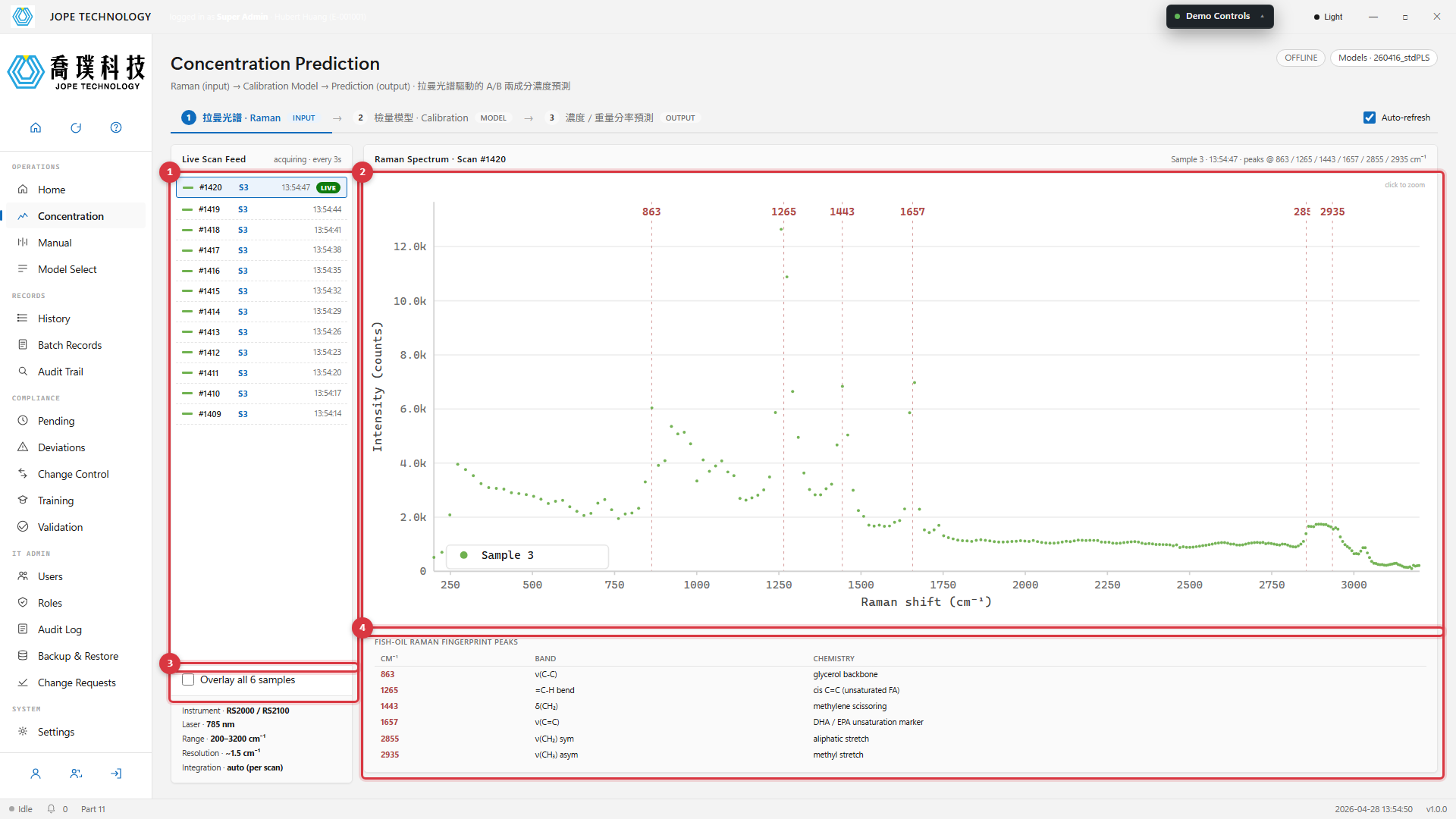
Figure 4.1 · Raman tab · Live Scan Feed on the left · current spectrum on the right · 6 fish-oil fingerprint peaks marked

1. Live Scan Feed · last 14 scans with scan number, sample, and timestamp
2. The highlighted row = the spectrum currently displayed
3. Red dashed verticals mark the fish-oil fingerprint peaks (863 · 1265 · 1443 · 1657 · 2855 · 2935 cm⁻¹)
4. Tick to overlay all 6 samples for comparison
5. The peak-table below the chart records the chemistry of each band

4.2 Calibration Model

Shows the PLS-Ridge calibration model file currently translating Raman spectra into concentrations. Each model file records training date, QA validator, RMSEP and R². This page is read-only — activation is done on the Model Select page.

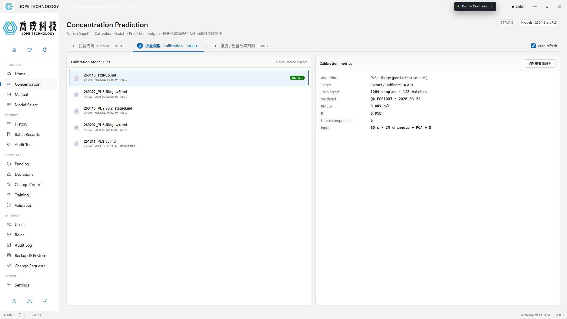
Figure 4.2 · Calibration tab · 5 model files with validation metrics and QA signature dates

4.3 Prediction (output)

Time-series of model output. Extract port (target Pure Strong A) and Raffinate port (target Pure Weak B) plot the A / B two-component concentrations in g/L. The header banner makes the source explicit: predicted by the currently active calibration model from live Raman scans, not a UV detector reading.

The Prediction tab has two sub-tabs:

• 3.1 Concentration · primary view, plots the live A / B concentration curves
• 3.2 Weight Fraction · reserved tab for the dynamic soft-sensor model output in wt% (currently a placeholder showing a "Coming soon" watermark and diagonal-stripe background)

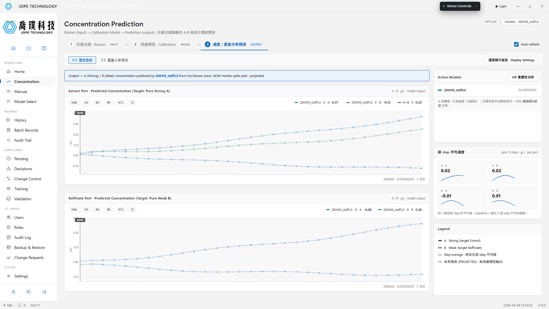
Figure 4.3 · Prediction tab · dual-port curves · 8 h history + 30 min projection · scroll to zoom / drag to brush

Line style conventions

• Solid line = component A (Strong); dashed line = component B (Weak)
• When multiple calibration models are active, each model uses a distinct colour (overridable in the Display Settings dialog)
• Horizontal short bars (line colour, semi-transparent thick stroke) = the step-average concentration for each completed step, useful for comparing consecutive steps
• The NOW vertical dashed line splits the chart into "past (calibration model output)" and "future (dynamic soft-sensor projection)"
• After NOW, the curve switches to fainter dashed lines + open dots, indicating projected values; the right panel shows a PREVIEW · soft-sensor pending chip

Future projection is not a measurement

The curve after NOW is a 30-minute projection from the dynamic soft-sensor model — informational only. Real-time control still relies on the live calibration-model output before NOW.

4.4 Weight Fraction Prediction (placeholder)

Switching to the 3.2 Weight Fraction sub-tab renders a diagonal-stripe background with a "Coming soon · awaiting dynamic soft-sensor model" watermark. Once the dynamic soft-sensor model is validated, this tab will switch to a real curve view in wt% units. The layout matches the concentration view so operators do not have to relearn it.

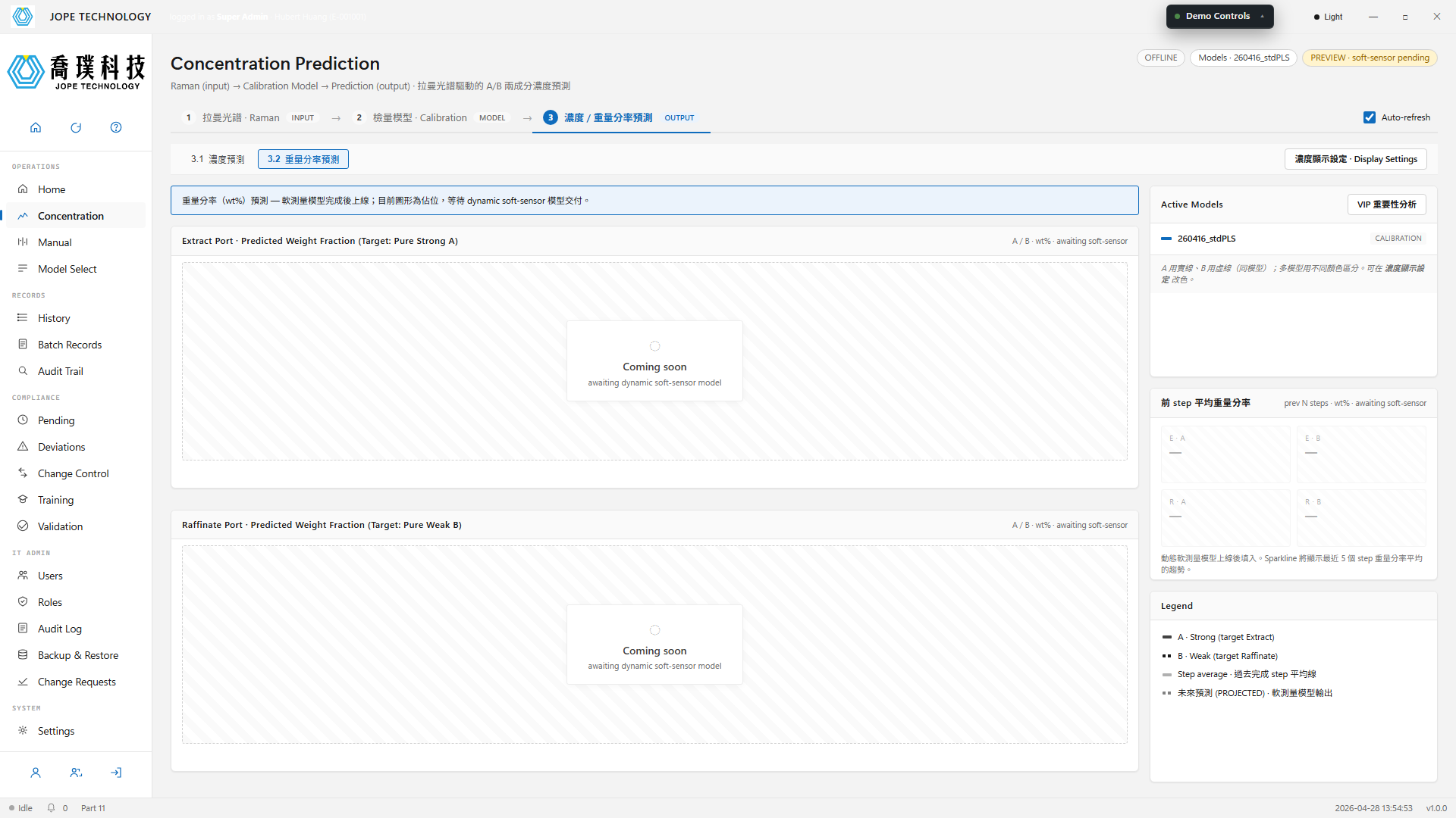
Figure 4.4 · 3.2 Weight Fraction · placeholder awaiting the dynamic soft-sensor model

4.5 Display Settings dialog

Click Display Settings (Chinese: 濃度顯示設定) to open the dialog. It controls three things at once: which targets to show, which models to use, and any custom summed traces to overlay.

1. Show targets · 2 × 2 table of checkboxes for Extract Port × A / B and Raffinate Port × A / B. Unchecking removes the trace from the chart immediately.

2. Active models · multi-select list of all available calibration models. Each row has a small colour picker — defaults to system-assigned colour, overridable when models need stronger visual distinction. Disabling a model greys out its colour picker.

3. Custom display content · three-column table:

   • Show · checkbox + Port (E / R) dropdown deciding which chart the summed trace is drawn on
   • Custom name · free-text label (e.g. A+B or Total)
   • Sum components · check the components to sum (A, B, or both)

   Three blank rows are provided. Enabled rows render as dotted (fine dashed) lines on the selected port chart.

4. Footer buttons:

   • Reset (初始化): restore all settings to system defaults
   • Apply (應用): apply the draft to the chart but keep the dialog open (for iterative tuning)
   • OK (確定): apply and close
   • Cancel (取消): discard the draft and close

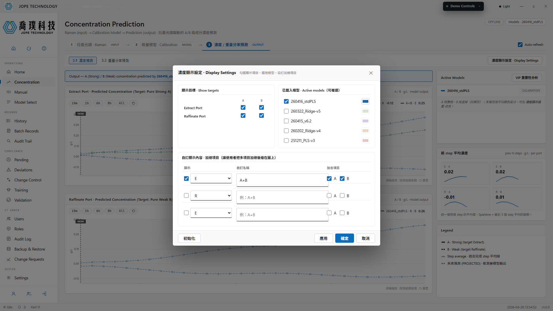
Figure 4.5 · Display Settings dialog · Show targets / Active models with colour picker / Custom sums / four footer buttons

4.6 Previous-step Average Concentration (stat card)

The Previous-step Average stat card on the right panel averages the predicted concentration across the most recently completed SMB step, plus a small sparkline of the last 5 step-averages. Operators use it to see whether successive steps are converging toward steady state.

This card and the in-chart horizontal bars present the same data two ways: the in-chart bars give visual step-to-step comparison; the card gives precise numbers and a recent trend. Both are governed by the Show targets setting (port × component combinations the user unchecks do not appear in the card either).

When switching to the 3.2 Weight Fraction sub-tab, the stat card auto-switches to a pending state (values display — with a diagonal-stripe background); real values populate once the dynamic soft-sensor model is online.

4.7 VIP Importance popup

Click VIP Importance Analysis on the Calibration Model panel at any time to inspect which wavelengths contribute most to the current model's prediction. The popup is non-modal, so the background concentration chart keeps refreshing.

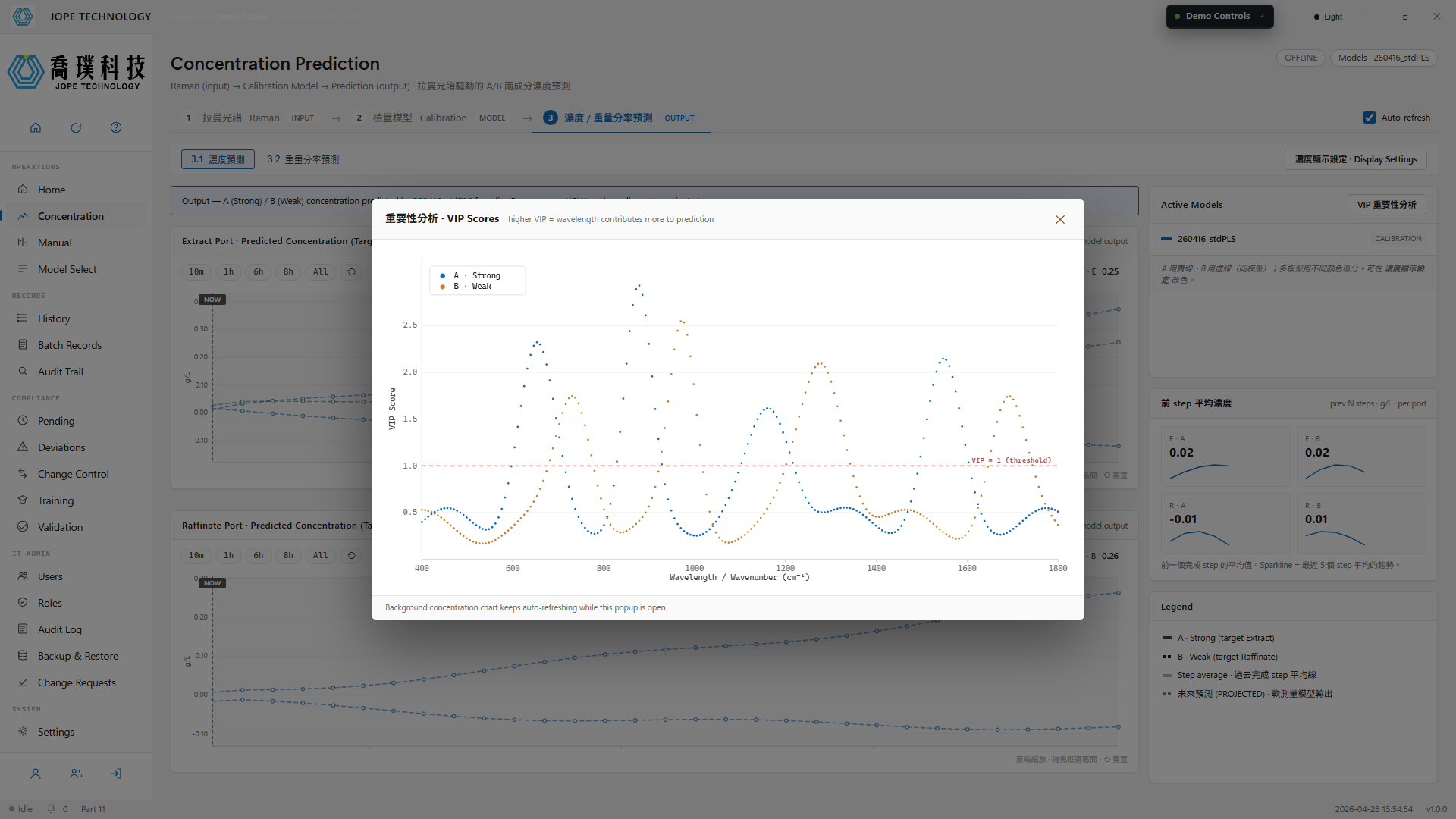
Figure 4.7 · VIP popup · VIP scores for Strong A and Weak B across wavelengths · threshold VIP = 1